Diffrentiation and integration

On the Sunday morning, I'd like make new post about Integral and diffrentiation

Calculus – differentiation, integration etc. – is easier than you think. Here's a simple example: the bucket at right integrates the flow from the tap over time. The flow is the time derivative of the water in the bucket. The basic ideas are not more difficult than that. Calculus analyses things that change, and physics is much concerned with changes. For physics, you'll need at least some of the simplest and most important concepts from calculus. Fortunately, one can do a lot of introductory physics with just a few of the basic techniques.
So stick with us: differentiation really is just subtracting and dividing, and integration really is just multiplying and adding. This short introduction is no substitute, however, for a good high school calculus course: we shall take some short cuts of which mathematicians may disapprove.

Differentiation: How rapidly does something change?

The velocity is the rate of change of displacement. Let's look at a very simple case. The strange man in this animation is moving in a straight line at a constant speed of one metre per second. This means that, for each second he travels, his displacement from the starting position increases by 1 m.
(An aside for physicists: velocity is a vector, meaning that it has direction as well as magnitude. So here we could say that his speed is 1 m/s but his velocity is 1 m/s towards the right. In these examples, we shall consider only motion in a straight line, so we can specify the direction simply thus: Positive velocity means going to the right, negative velocity means going to the left. By the way, the magnitude of velocity is called the speed, which we could write as |v|. Speed is a scalar, velocity is a vector. See vectors to revise.)


When the clock strikes zero, he is at x  =  3 m. We call this his initial displacement and write x₀  =  3 m.
When the clock reads t  =  2 s, he is at x  =  5 m. So what is v? Displacement has increased by 2 m, time has increased by 2 s, so v is

Now this is a special case, because in this example he is travelling at constant speed. Let's see how special: What if he travelled at 2 m/s for half a second, stopped for one second, then travelled at 2 m/s for another half second? He would still have travelled two metres in two seconds, so his average speed would be 1 m/s, even if he were never travelling at this speed. We signify the average of something by putting a bar over it. His average speed is written , pronounced 'v bar'.

That fraction above looks long and clumsy when written in words. We'll write x for displacement and t for time. "change in" occurs so often in physics that we replace it with the Greek letter delta, whose upper and lower case forms are Δ and δ. (In a word, δ sounds similar to the 'd' in English, so you can think of it as standing for 'difference'.) With that substitution, and remembering to use average velocity, we write: Now, don't get too excited, but what we have just done is called 'differentiation' or 'taking a derivative'. Yes, that's all there is to it: we subtracted to obtain a difference, and divided it by another difference. That process is called numerical differentiation, and most differentiation is numerical. Note the geometrical significance of taking the derivative: looking at the triangle drawn on that graph, the height is 2 m, and the base is 2 s, so the derivative is the slope of the graph. Often it is said to be the rise (here Δx) over the run (here Δt). 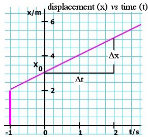Note too that, for this case, it doesn't matter how big or where we draw the triangle. If we made the run 0.3 s, the rise would be 0.3 m, and so on. That, however, is just for this special case, where v is constant, and so v and are the same. The derivative of x in this case is constant, as we show in the v(t) graph above.

Varying derivatives

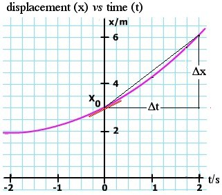
What if v is not constant? Here's a simple case in which the same bloke is accelerating forwards, so his velocity is increasing. Let's work out his velocity at any particular time t, just from the graph x(t). We want to find the slope of this curve, at different values of t, as is shown in the animation. How can we do it? Well, in most cases, and especially in the case of experimental measurement, we do the same thing that we did for the simple case: we draw a triangle and put change in displacement Δx over change in time Δt. Again, this is numerical differentiation.

If we want the slope at t  =  0 s, we might take t  =  0 s and t + Δt  =  2 s. So Δt is two seconds, using the notation introduced above. But the trouble is that that gives us a triangle whose slope (the black line) is somewhat greater than the slope at t  =  0 s (the red line). In fact, the slope of the black line gives us the average velocity between 0 and 2 seconds, but that is not what we want. We can do better, in this case at least, by drawing our triangle on either side of t  =  0 s. Try it, but you'll find that that gives an overestimate, too. We can do better by taking a smaller value of Δt. At first, we expect the estimate to improve as we take smaller and smaller Δt. Here arises a practical problem: If we are measuring the values, there is inevitably a limit to the precision of each measurement and, as the Δt and Δx get smaller, this error becomes proportionately more important. If we are calculating x and t numerically, we face the same problem. So, in practice, we make a compromise on the size of Δt: small enough to give the local shape of the curve but large enough that the measurement or calculation errors are small. There are other tricks that we'll see below.

Analytical derivatives

But what if we 'know' the formula for the function x(t)? I have put 'know' in quotation marks, because for anything in physics, the only things that we know are the measurements. There are only a finite number of these, so we just have a set of points on a graph. What we can do is to find a mathematical model, a formula that goes close to the points on the graph. For example, if the acceleration is constant, we might use x  =  x₀ + v₀t + ½at², as we do in the chapter on constant acceleration. We can now choose whatever t we like, and calculate x to whatever precision we need, though of course the final precision will depend on how well we know x₀, v₀ and a, so we are still limited by measurement.

Power terms and polynomials

Let's have a look at these terms in turn. If x  =  x₀, then it's simple: no variation in x, so the derivative would be zero. What about x  =  v₀t, in other words constant velocity? This is like the first example we did: the derivative is constant, and it equals v₀. So, the derivative of a constant is zero, and the derivative of a term that is proportional to t is just the constant of proportionality or, in standard terms, the coefficient of t. But what of a term like x  =  Ct²? (In our example, C  =  a/2, but let's keep it general.) Let's make the 'run' for our slope calculation from t to (t+Δt). Then the 'rise' on the triangle will be from Ct² to C(t+Δt)². So the slope is

Now let's make Δt and Δx extremely small, and we signify this by writing them as dt and dx.
As we've said, dt is very small, and can be made smaller than anything that we could measure. So we can neglect it on the right hand side. We don't neglect it on the left hand side, because there we have the ratio of two small things, and that ratio need not be small. So here we have one useful case for taking derivatives: the derivative of Ct² is just 2Ct.

At this stage, if you were doing this in a mathematics school, you might start to worry about infinitesimals, and taking the limit as Δt goes to zero. I may get into trouble for pointing this out, but the universe doesn't have infinitesimals, and quantities don't go to zero in physics. Infinitesimals, like many things in mathematics, are human inventions. So, for most purposes in physics, the limit taken is just the size necessary to have mathematical precision greater than that of our measurements, or greater than that of our numerical calculation. (You really should take that mathematics course, but you won't need infinitesimals in physics.)
Let's summarise what we have so far:
Let's graph these, setting the constants equal to one. We'll also omit units on the axes because, although you may find it helpful to think of the vertical axis as displacement and t as time to give a concrete example, the results are general. For that reason, we'll use y as the vertical axis from here on. In all of the graphs on this page, the red curve is the derivative of the purple one. It is a good exercise to compare the two, and to check that, in all cases and over the whole curve, that the red line represents the slope of the purple one. Here, for instance, the slope of y  =  1 is zero. The slope of the straight line y  =  t is obviously consant. In the third curve, you can see that the slope is negative at first, zero at t  =  0, and then becomes increasingly positive.

Perhaps you see a pattern here? Taking a positive integer n, and expanding (t + Δt)ⁿ, you'll see that, if y   =  Ctⁿ, the derivative of y is nCtⁿ⁻¹. This is often written thus:

This result is more general: it actually holds for all real values of n, positive and negative. n  =  0 is a special case, because it gives a factor of zero on the right hand side. This will be important when we come to look at integrals, below.

Sums of terms

If x is increasing with rate (dx/dt) and y is increasing with rate (dy/dt), what is the rate of increase in (x+y)? This is an easy one: if, over a certain time t+ Δt, x increases by Δx and y increases by Δy, then the change in (x+y) is (Δx+Δy). The rate of change in the sum of functions is equal to the sum of their individual rates of change. (The derivative of the sum is the sum of the derivatives.) With this unsurprising result, we can now differentiate polynomials, such as this: If

y  =  A + Bt + Ct² Dt³, then
dy/dt  =  B + 2Ct + 3Dt².

Trigonometric functions

Sine and cos functions are important, especially in circular motion, simple harmonic motion, components of forces and other cases involving components of vectors. Fortunately, the derivatives here are simple. Let's work them out, using this diagram, which shows a segment of a circle whose radius is one unit. (We say a circle of unit radius.) The definition of sine of an angle uses a right angled triangle. It is the ratio of the side opposite the angle to the hypotenuse of the triangle. The definition of cosine is the other side (that adjacent to the angle) divided by the hypotenuse. In this diagram, first look at the triangle with blue sides. The radius is drawn at the angle θ. The vertical side is, by definition, sin θ and the horizontal side is cos θ. Now let's change θ by an amount Δθ: we get another radius and another triangle, shown here with two of its sides in green. By how much have we changed sin θ? In other words, what is Δ(sin θ)? By definition, Δ(sin θ) is the amount that in θ increases when θ increases by Δθ). So it must be (sin(θ+Δθ) − sin θ). On this diagram, Δ(sin θ) is shown as the rise of the small triangle, shown in red. (For clarity, this triangle is repeated outside the main diagram.) The run of this triangle is −Δ(cos θ). The run goes to the left in this case, so it has a negative sign. This negative sign arises because, as θ increases in this quadrant, cos θ decreases. Now look at the small right triangle in red. We call its hypotenuse h. Applying the definition of sine and cos, and remembering that the cos θ is decreasing, we have Δ(sin θ)  =  h cos φ      and      Δ(cos θ)  =   − h sin φ. Now let's imagine what happens to the little red triangle as Δθ becomes very small. The hypotenuse approaches more and more closely the length of the arc of the circle between the two radii (the radii are the blue hypotenuse and the green hypotenuse). From the definition* of angle (angle in radians ≡ arc/radius) and the fact that radius is one, this arc has a length Δθ. It follows that, as Δθ becomes very small, h becomes approximately Δθ. Further, h becomes closer and closer to being at a right angle to the radius. Further, the angle φ becomes closer and closer to being equal to θ. Again, we use the convention that dx means a value of Δx small enough to make the approximations better than our measurements. So, in this limit, and using the results of the previous paragraph (θ  =  φ and h  =  dθ for small enough values of Δθ), the equations above become d(sin θ)   =   dθ cos θ     and     d(cos θ)  =   − dθ sin θ Dividing both sides of these two equations by dθ gives two very useful results: * Note the use of the definition: angle in radians  =  arc/radius. Consequently, the dθ in these equations must be expressed in radians. To convert degrees into radians, multiply by π and divide by 180°.

The chain rule

Suppose we have a function z that depends on t, in a way that allows us to calculate z if we know t. And suppose that x depends on z in a similarly explicit way. Just by cancelling a factor, we can write:
If all of these are very small quantities, then we write
This is the chain rule of differentiation, which we use when analysing circular and simple harmonic motion.

Circular and Simple Harmonic Motion

In both these cases, we consider uniform circular motion, in which the angle θ increases linearly with time, so (dθ/dt) is a constant, called the angular velocity ω. We can write this as
θ  =  ωt + φ
where ω is constant and where φ is the initial value of θ. We therefore write for the vertical displacement
y  =  A.sin θ  =  A.sin (ωt + φ),
When we take the time derivative of θ, we have dθ/dt  =  ω. So the chain rule gives:
v_y  =  dy/dt    =  (dy/dθ).(dθ/dt)  =  (A.cos θ).(ω)   =  A.ω.cos (ωt + φ).
So much for maths: where, physically, does the extra factor ω come from? If we double ω, we double the rate at which the angle is increasing in circular motion or the phase is increasing in simple harmonic motion. So the time for one complete circle or cycle is halved. If the displacement goes through the same variation in half the time, then the velocity is doubled. (Differentiating one more time gives an acceleration that includes, in both cases, a factor ω ². So, if we double ω, the range variation in velocity is twice as great, and we go through that range twice as often, so the acceleration has an extra factor of 4.)

---

Integration: How do the results of a variable rate add up?

Let's leave displacement time graphs for a moment, because my favourite example of an integrator is a bucket. A bucket integrates the flow of water from a tap above it. In our example, someone is turning the tap on an off in an erratic way, so that the volume flow f (measured in litres/second) is varying with time. That function f(t) is shown as the red curve in the figure. Let's say that the bucket already has in it a volume V0 of water and that we put the bucket under the tap (we start integrating) at time t  =  0. The tap is already on, with a flow rate f0, called the initial flow rate. Consider the first short interval Δt. The flow rate is by definition the volume per second so, in the first time Δt, a volume of approximately f0.Δt pours into the bucket. f0.Δt is shown by the first red rectangle on the top graph. "Approximately" is there because, during Δt, the flow is not constant, but varying – in our example it is increasing. 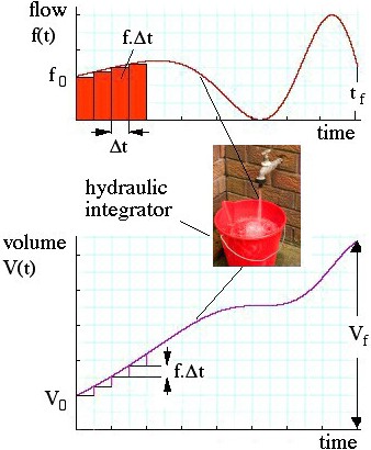Similarly, at any time later, the volume going into the bucket in the short interval Δt is approximately f.Δt. So, for each Δt we add a step of f.Δt to the height of the purple curve representing the volume in the bucket, as shown in the lower curve. Notice that, when the flow is high, the area f.Δt is large, so that is when the volume in the bucket increases rapidly. Note that, when the flow falls to zero (tap off), the volume is no longer increasing. And of course a fall in the V(t) curve would mean water flowing out of the bucket, which we should call negative flow into the bucket. (For example, the bucket might have a leak.) What is the volume Vf in the bucket at a final time tf? (The subscript f here stands for 'final', not flow.) We can find the approximate volume as Vf   ≈   V0 + f0.Δt + f1.Δt + f2.Δt + etc until we get to tf. The "approximately" appears because the flow varies over the time Δt. However, if we make Δt small enough, this variation becomes smaller than the limit of our precision*. As above, when Δt is small enough, we call it dt. So the equation above becomes: Vf   =   V0 + f0.dt + f1.dt + f2.dt + etc until we get to tf. So the right hand side has the initial volume, plus a long sum of terms like f.&dt. That sum is called the integral of f with respect to t. We saw earlier that differentiating was subtracting and dividing. We've now seen that integration is just multiplying and adding. So integration is the opposite of differentiation. The language we've used above includes "+ etc until we get to tf and where dt is small enough to achieve the required precision". We'd waste time (and look a bit silly) writing this every time. So instead we write it like this: The last term is pronounced "The integral from t = 0 to tf of f with respect to t". The integral sign is s shaped, which can stand for 'sum' and remind us that's all it is. We say we are integrating "with respect to t", because t is varying during our sum. The limits of integration (t = 0 and t = tf) tell us when we start and stop integrating – when we put the bucket under the tap and when we pull it away from the tap. In the way I've presented this example, V0 is a constant of integration. Integration doesn't tell you the complete answer, it only tells you how much something has changed during the process. In this case, to know the final volume in the bucket, we need to know not only the integral of the flow, but also how much was in the bucket before it started to integrate the flow. In most cases, you will need to find the constant of integration – very often by using the initial conditions, as we did here. Perhaps now is a good time to go back to the animations above and check that integrating the velocity (finding the area under the curve) gives the displacement.

Numerical integration

If we had a set of numerical values for f(t) – whether experimental values or values calculated for a given mathematical function – then we could integrate just as described above: mutliple f by Δt and add. That's what my pocket calculator does when I hit the "∫" key. You've probably thought that it would be smart to space the limits of Δt on either side of the time whose value you used to get f: that's a good idea and you should remember it when you have to do a numerical integration. A very important practical point: when we made Δt small in differentiation, we encountered the problem that the ratio Δx/Δt became sensitive to experimental or computational error as Δt became small. This problem does not arise in multiplication. Even better, the computation errors, being sometimes positive and sometimes negative, tend to cancel out. So numerical integration is much easier and safer than numerical differentiation. The latter requires considerable caution (and that is why my calculator doesn't have a "differentiate" button).

Analytical integration

This section might be shorter than you expect. We've mentioned above that integration is the opposite to differentiation:
The rate at which something changes is its derivative, but
You can recover that something by integrating the rate at which it changes. In differentiation, we subtract V(t) from V(t+dt) and divide by dt
In integration we multiply f(t) by dt and add it to V(t), where f is the derivative of V with respect to t.
So for analytical integration, we can use in reverse the tricks we established above for differentiation. Omitting constants of integration, we write
The derivative of tⁿ is nt^n-1, so
The integral of nt^n-1 is tⁿ
provided that n is not equal to zero, because in that case the first equation gives us no information. Dividing the last equation by n, and substituting m  =  n−1 gives

• The integral of t^m is t^m+1/(m+1)
when m is not equal to −1. This is an important exception, which we'll deal with below.

The exponential function

One very useful integral and differential is the exponential function. The function e x is chosen and the value of e defined so that the derivative of e x is e x. In other words, e x is a curve whose slope equals its value at all points. So it is also its own integral. On the graph, the curve (purple) shows e x vs  x. In this the derivative is not shown in red, because the function and its derivative are equal. The straight line (green) is y  =  e x. At x  =  1, the slope of the curve is e 1  =  e . This is also the value of y at x  =  1. Notice that, at x= 0, the slope of the curve is one. At x  =  −1, the slope is 1/e , etc. Using the chain rule tells us that The derivative of e ax is a.e ax, where a is a constant, and The integral of e ax is e ax/a. To return to our point about numbers and physical quantities: Be careful about dimensions: the argument of the exponential function must be a number. Consequently, in physics, we shall often see the exponential function in equations like this one for a displacement decreasing exponentially with time: x  =  x0.e −t/τ where x0 is the displacement at t  =  0 and τ, which must have the units of time, is the characteristic time that appears due to parameters in the physical system. This example suggests a nice problem: what is the relation ship between force and velocity for a particle of mass m whose velocity is given by v  =  v0.e −t/τ where v0 is the initial velocity? And how far does it travel before coming to rest? (This situation occurs for an object moving slowly and horizontally without friction in a viscous medium. For object moving rapidly, the retarding force is approximately proportional to the square of the speed. See the integral in car physics.)

1/x and the log function There was an exception above, and there is one here. Obviously this can't work for m  =  −1, because that would give an integral that doesn't depend on t. The integral of 1/x is ln (x). Let's see why. (If you need to, see What is a logarithm? A brief introduction, below.) Let's put y  =  ln x. So by definition that means x  =  ey Let's take derivatives, remembering that the exponential function is its own derivative: dx/dy  =  ey  =  x Now divide both sides by x and multiply by dy to obtain dx/x  =  dy But above we defined y   =  ln  x, so dx/x  =  d(ln x) Remember this one – you'll use it a lot. So, in the plot at right, the purple curve is y  =  ln x. Its slope (the rate at which it is increasing) is given by the red curve (dy/dx  = 1/x). Alternatively, we could say that the purple curve rises at a rate given by the red curve (integration of a function means successively adding its value). For this and later sections, you'll notice that the examples use numbers x and y, rather than displacements as a function of time. Quantities with dimensions add extra constants, as we see below, and it is easier to begin without them.

The integral of sine and cos

Above we saw that the derivative of sin θ is cos θ, and the derivative of cos θ is − sin θ. So
• The integral of cos θ is sin θ, and
• the integral of sin θ is − cos θ.

Techniques for integration

You need to assemble a little collection of integrals of simple functions, including those listed immediately above. There is a range of techniques for integrating more complicated expressions. In approximate order of frequency, these are the techniques I use:
• Change the variables to make it more closely resemble an integral I do know. Here are a couple of examples:
  • to integrate dx/(1+x), try the substitution y  =  1 + x. Here dy is equal to dx, so this gives an integral we've seen above: dy/y = d ln y.
  • to integrate x.dx(1 − x²)^−1/2, which arises in different areas of physics, try the subsitution x  =  sin θ. We can now write (1 − x²)  =  cos θ, and dx  =  cos θ.dθ. Wow, that now looks much easier! (This is just one of a whole family of trigonometric substitutions.)
• Integrate by parts. This technique comes from the derivative of the product of two functions. (This is getting beyond what we need for the material here, so see a book on calculus for more details.)
• Look up a table of integrals! These have pages and pages of integrals, which are presumably assembled "the other way round" – i.e. the authors probably make a table of derivatives, then index it in terms of the integrals. Here's one on Wikipedia.
• Try an algebraic mathematical package. (Where this is useful, it often makes you feel like a dill for not having seen it yourself.)
• Integrate numerically – for many problems, this is the only way.